Calibrating the Compass - Part I

To start to understand the readings from the MiniMu-9, and to calibrate the device, I conducted a simple experiment.  Place the Raspberry Pi on a flat surface, align it with my iPhone so that the Compass app points North, and run my Capture Python program to study the compass data.  Here's the output:

That's confusing.  Firstly, it looks like the second registers (X1, Y1, Z1) don't do anything except indicate an overflow of the lower register.  Next, there's pretty significant variation in the readings for a device that's sitting still on a table top.  From 20 readings, the variation in the lowest register base 256 is:

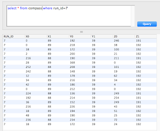
Xmin = 42, Xmax = 132, Xrange = 90

Ymin = 102, Ymax = 232, Yrange = 120

Zmin = 197, Zmax = 76, Zrange = 135

Now if one in the upper register is 360/256 degrees then that's maybe not too bad.  Looks like I have some work to do with the MiniMu9 documentation to understand the readings.

Here are the application notes for the compass chip.

"Understanding magnetic data The magnetic data are sent to the OUT_X_H, OUT_X_L, OUT_Y_H, OUT_Y_L, OUT_Z_H, and OUT_Z_L registers. These registers contain, respectively, the most significant part and the least significant part of the magnetic signals acting on the X, Y, and Z axes."

Not so helpful guys ... what do the numbers mean.

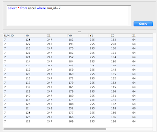
Let's resort to trial and error.   With the device on the same table, rotating it 180 degrees to face South, here is the corresponding data:

It appears that my Y1 and Z1 values have not changed, but by rotating the device 180 degrees, my median X value has changed from 246/87 to 2/250.    Now, assuming the lower register represents the 8 least significant bits of a 16 bit number

An alternative way of looking at this is that by rotating 180 degrees, the median magnetometer X reading has changed from (246*256)+87=  63,319 to (2*256) + 250 = 762.    

OK, so I need to apply some scientific method.  I've four questions that I wish to answer:

1.  Is the compass behaving in a stable manner, or is it just sending random signals?
2. Does the compass signal behave in a way that is stable over the average of a series of readings, and if so, how long does the series have to be?
3. Is angular change represented linearly by the magnetometer readings?
4. How are the X, Y and Z axes oriented compared to horizontal and North?

To research the answers to these questions I ran my Python code to collect a series of 200 readings with the Raspberry Pi oriented in 36 positions at 10 degree increments starting at North.  The readings were taken on the same position on a smooth leveled surface.  I measured the 10 degree increments using a military compass, as I noticed that the iPhone compass could jump by as much as 30 degrees without the iPhone being moved.

Ideally the data gathering would have been done on a carefully leveled surface, using a carefully calibrated turntable to rotate the sensor.  I'm not expecting fantastic results, but let's take a look before I start spending on a calibration rig.

As the data were written to the SQLite database, the 10 degree run was assigned RUN_ID=17 with the RUN_IS incrementing by 1 until the 360 degree (North) run was assigned RUN_ID=52.

Analysis of Calibration Data

I took the data from the above runs and imported it into an R data frame using the RSQLite library:

library("RSQLite", lib.loc="~/Library/R/3.2/library")
library("ggplot2", lib.loc="~/Library/R/3.2/library")

c <- dbConnect(SQLite(),
        dbname="/scratch/sqlite3/sensors.sqlite")

d <- dbGetQuery(c, "select * from compass where run_id >= 17")

I then merged the values from the two registers, and adjusted the values where they had wrapped around 2^16 and started again at zero:

d$X <- (d$X1 * 256) + d$X0
d$Y <- (d$Y1 * 256) + d$Y0
d$Z <- (d$Z1 * 256) + d$Z0

# improve visibility by fixing the wrap around 2^16
d$X <- ifelse(d$X < 2^12, d$X + 2^16, d$X)
d$Y <- ifelse(d$Y < 2^12, d$Y + 2^16, d$Y)
d$Z <- ifelse(d$Z < 2^12, d$Z + 2^16, d$Z)

# Convert Run ID to a factor to improve color coding
d$RUN_ID <- factor(d$RUN_ID)

I then created a summary data set, showing the mean, median, sd, max and min values for each run.

library("plyr", lib.loc="~/Library/R/3.2/library")
Xsum <- ddply(d, "RUN_ID", summarize, Xavg=mean(X), Xmed=median(X),         Xsd=sd(X), Xmin=min(X), Xmax=max(X), Xspread=max(X)-min(X))
Ysum <- ddply(d, "RUN_ID", summarize, Yavg=mean(Y), Ymed=median(Y),         Ysd=sd(Y), Ymin=min(Y), Ymax=max(Y), Yspread=max(Y)-min(Y))
Zsum <- ddply(d, "RUN_ID", summarize, Zavg=mean(Z), Zmed=median(Z),         Zsd=sd(Z), Zmin=min(Z), Zmax=max(Z), Zspread=max(Z)-min(Z))

# join dataframes
XYsum <- join(Xsum, Ysum, by="RUN_ID")
XYZsum <- join(XYsum, Zsum, by="RUN_ID")

Visualizations of Calibration Data

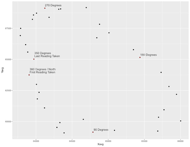
I then used ggplot2's qplot function to visualize the averages of X and Y for each set of readings.  Ideally the data should form an ellipse.   The shape of this ellipse will help us calibrate the compass.

qplot(data=XYZsum, x=Xmed, y=Ymed)

Note, the annotations were added using Affinity Designer and were not generated by qplot.

It's moderately elliptical.  It's clear that the act of rotating skews the readings as there's a clear disconnect between the first and last readings.  There are also potential sources of error arising from:

• the compass reading
• aligning the box of the Raspberry Pi with the edge of the compass
• local magnetic variations (movement of people and objects close to the Raspberry Pi)
• very large outlier readings which are skewing the mean.

To minimize the last of those problems I re-ran the chart using the median instead of the mean for each position of the Raspberry Pi.  There really was not much difference between the two.

From here we should be able to draw a best fit ellipse through the data points, which can then be used to interpret future readings.

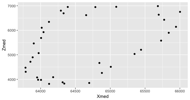
We can also repeat this for the XZ readings to interpret the angle in the XZ plane.  The chipset documentation says that the Z axis is perpendicular to the plane of the board, which would make Z independent of rotation about the XY plane, which would result in a horizontal flat line.  But we already know that the chip is mounted slightly off because the XY rotation resulted in an ellipse and not a circle.  The XZ plot should therefore also result in an ellipse:

Again, not too pretty an ellipse, but for now lets assume that the errors arose from my non-scientific data gathering.

Before I do that, let's think about the variation in the readings within any given run, and how many readings we need to take to be sure we have an accurate compass reading.

Sampling Analysis

The first thing I noticed is that the Standard Deviations are quite small compared to the range.  A typical example is the X readings for the 10 degree run.    Of the two hundred readings:

• the mean is 64,006.7
• the median is 64,007
• the standard deviation is 28.1
• the minimum is 73 less than the median
• the maximum is 75 more than the median

The readings are not widely dispersed, with all readings being within 3 standard deviations of the mean.   Now, each of these readings was taken 0.1 seconds apart with the device standing still.  My concern is that we will not have the opportunity to take a large number of readings spaced apart like this - a skier's direction will be rapidly changing.  If I take a smaller number of readings more closely spaced, will I get a similar spread to calculate a good median without the skier moving too far during the sample?  To test this I wrote a variation of the sampling code to take 30 samples immediately after each other.

Taking 30 samples only 0.1 seconds apart I get:

• median is 65,778
• the minimum is 34 less than the median
• the maximum is 36 higher than the median

Reducing the sampling period to 0.01 seconds I get:

• median is 65,809
• the minimum is 57 less than the median
• the maximum is 67 higher than the median

Eliminating the sample wait altogether I get:

• median is 65,827
• the minimum is 241 less than the median
• the maximum is 207 higher than the median

I repeated this a number of times and the principle seems to hold, that if I do not wait between samples then I get bigger errors in the lower register.  Increasing the wait to 0.5 seconds does not further reduce the error rate.  Wait times in the range 0.05 - 0.1 seconds appear to have generally similar results.

It seems that I will have to accept inaccuracies in the direction measurement.  If I take the median of ten samples 0.05 seconds apart, then I can only capture data every 0.5 seconds which is not sufficiently frequent for my needs.  If I sample more frequently then the errors get larger, with the consequent risk that a small number of samples will not provide an accurate median.  For now I will proceed with the approach of taking only a single sample of each reading, and having readings no closer than 0.05 Seconds apart, and will pay attention later to whether the noise in the readings detracts from the end result.

Fitting an Ellipse

Using the least squares fit method for fitting an ellipse to data, and the accompanying R code in Reference B, I fitted an ellipse to the data generated by the X and Y magnetometer sensors.

I found two problems with the results of the R code:

• The angle of rotation is off by 90 degrees (pi/2 radians).  
• The fit is not particularly good when using large coordinates.

My sensor had created most values just below the maximum value of 2^16, but in a few cases had wrapped over the maximum 2^16 values and used values just over zero.  I previously adjusted for this by adding 2^16 to any values that are less than 2^12.  Because the ellipse matching works better with values centered on zero I now altered my coordinates by subtracting 2^16 from all of them.

I also arbitrarily added pi/2 to the angle of rotation to correct for that issue.

Incidentally, I encountered the same rotation issue when trying the Python code in Reference C.  I also found with the Python code that the ellipsis semi-axes lengths were miscalculated with large coordinate values, and this issue was resolved when I subtracted 2^16 from all x and y values.

Here's my R code (I have not repeated the functions fit.ellipse and get.ellipse, which were used unaltered from the reference:

xy <- data.frame(XYZsum$Ymed, XYZsum$Xmed)

colnames(xy) <- c("x", "y")

xy$x <- xy$x - 2**16

xy$y <- xy$y - 2**16

xyfit <- fit.ellipse(x=xy$x, y=xy$y)

xyfit$angle += pi/2.0

xyElipseCoords <- data.frame(get.ellipse(fit = xyfit, n=360))

qplot(data = xy, x=xy$x, y=xy$y, color=I("red"), c(-2000, 1000), ylim = c(-7000, 4000) xlab = "x", ylab = "y") +

geom_point(data = xyElipseCoords, x=xyElipseCoords$x, y=xyElipseCoords$y, color="blue", shape=1)

And here's a plot of the original data in red and 360 data points on the fitted ellipse in blue:

Next I will take the 360 data points of the fitted ellipse and store them in a Python list with the point relating to North in the 360th position in the list.  Thereafter, if I create a function to identify the closest point in the list to a sensor reading, then its position in the array will represent an angle in degrees in the XY plane, ie a compass heading.

I can also repeat this approach for the XZ plane and the YZ plane.

.import pandas as pd


def find_closest_pair(x, y, ref):
    # ref is dict of the form {1: {x: 1, y: 2}, 2: {x: 3, y: 4}}
    residuals = {}
    for key in ref:
        pt = ref[key]
        residuals[key] = (pt["x"] - x)**2 + (pt["y"] - y)**2
    min_error = min(residuals.values())
    for key in residuals:
        if residuals[key] == min_error:
            min_error_posn = key
    return [min_error_posn, min_error]

df = pd.read_csv("/Users/neildewar/scratch/xy360.csv")
ref = {}

for index, row in df.iterrows():
    ref_pt = {}
    ref_pt["x"] = float(row['x'])
    ref_pt["y"] = float(row['y'])
    ref[index] = ref_pt

closest = find_closest_pair(-1784, -1634, ref)

print(closest)

Now, that might be a lot of work to find out that True North is already stored in the last item in the array, but the function called find_closest_pair() will be re-used later on the Raspberry Pi when I need to match new sensor readings to return a direction in the XY plane.

References

A. Useful article on interpreting magnetometer readings: http://mythopoeic.org/magnetometer/

B.  Article on best fitting an ellipse to data, providing R code: https://www.r-bloggers.com/fitting-an-ellipse-to-point-data/

C. Article on best fitting an ellipse to data, providing Python code: http://nicky.vanforeest.com/misc/fitEllipse/fitEllipse.html

Getting my Raspberry Pi mobile

In order to start using my sensors on the move I need to solve two mobility problems:

• Provide a mobile power source (it's currently powered from mains)
• Securing the sensor in the Raspberry Pi's case so that it's always in the same orientation to the case.

Mobile Power

I hunted around my office and found one of those cell phone emergency re-chargers that I had been given at a conference.  The unit was a good sized one and should be able to run the Pi for a few hours.  It's a RedFuel SL5.

The power unit comes with a cable that has a regular USB connector on one end, and a D port on the other end.  It charges by plugging the USB end of the cable into a transformer, and the D connector into the port on the right of the above picture.  When it's fully charged, the cable is turned around so that the USB end is plugged into the RedFuel power unit and the D connector is plugged into the Raspberry Pi's power port.

Securing the Sensor

To get consistent readings it will be important that the MiniMu-9 card is secured to the Raspberry Pi with a consistent orientation in all three dimensions.  The MiniMu-9 board is not easily secured to the Raspberry Pi.  I considered using an stand-off connector, but all four holes on the Raspberry Pi are used to secure it to its case.  I decided to glue the cable connectors (not the board!) to the inside of the removable roof of the Rapsberry Pi.  The cable coil away nicely inside the case.  Here's the whole installation:

A SQL Database To Store The Data

Creating The Database

I used a copy of the Mac app SQLite Manager to create my database.  I chose a simple relational model with four tables.  The first table is to store details of the "run" ie a sequence of sensor readings.  There are then three tables to store the actual readings from the gyro, accelerometer and compass respectively.  Each of the three sensor tables includes a column that indicates the run that the sensor reading was associated with.

Each of the sensor tables contains six integer fields (X0, X1, Y0, Y1, Z0, Z1) to store the values that were read from the sensors.  They also have three float fields (X, Y, Z) to store the numeric values after the readings have been processed and calibrated (more to follow on that later). 

Writing Data to The Database

First a word of caution, close the SQLite Manager app before programmatically writing to a database.  It has a nasty habit of crashing.

I wrote the Python code in Python 2.7.4 using the PyCharm Community Edition (ie free) IDE.

I have included python code below to write to the database.  It is pretty straightforward.  It uses three libraries:

• The json library to parse the data that is stored in the data file.
• The sqlite3 library to make the database connection to the sqlite database.
• The os library allows interaction with the file system to change directory.

The python code then performs the following tasks:

• Create the database connection
• Open the JSON file that was created on the Raspberry Pi containing the sensor data
• Read the JSON file and write it to the database tables
• Read the header information to create a run record, and capture the RUN ID
• Loop through the readings data, processing each in turn
• Read Gyro data and write to DB
• Read Accel data and write to DB
• Read Compass data and write to DB

A few words on the sqlite code:

• You initiate a connection to the database, that returns a connection object
• The connection has a cursor object.
• The cursor object is used to execute SQL commands against the database
• The connection object is used to commit the SQL commands.

This website is very helpful on how to use the sqlite from Python.

import json
import os
import sqlite3


def init_db(db_file):
    conn = sqlite3.connect(db_file)
    return conn


def load_file(filename, filedir):
    os.chdir(filedir)
    f = open(filename, "r")
    d = json.load(f)
    return d


def process_header(header, db):
    c = db.cursor()
    # expects dict of the form {"type": "header", 
                             #  "Month": 12, 
                             #  "Day": 4, 
                             #  "Year": 2016}
    c.execute("INSERT INTO RUN (Year, Month, Day) 
              "values ({yr}, {mth}, {day})".
        format(yr=header["Year"], 
               mth=header["Month"], 
               day=header["Day"]))
    db.commit()
    return c.lastrowid  # return the PK of the last row entered

def process_reading(reading, db, header):
    c = db.cursor()
    accel = reading["accel"]
    c.execute("INSERT INTO ACCEL (RUN_ID, x0, x1, y0, y1, z0, z1) "
              "values ({hdr}, {x0}, {x1}, {y0}, {y1}, {z0}, {z1})".
        format(hdr=header,
               x0=accel["x0"],
               x1=accel["x1"],
               y0=accel["y0"],
               y1=accel["y1"],
               z0=accel["z0"],
               z1=accel["z1"]))
    db.commit()

    gyro = reading["gyro"]
    c.execute("INSERT INTO GYRO (RUN_ID, x0, x1, y0, y1, z0, z1) "
              "values ({hdr}, {x0}, {x1}, {y0}, {y1}, {z0}, {z1})".
        format(hdr=header,
               x0=gyro["x0"],
               x1=gyro["x1"],
               y0=gyro["y0"],
               y1=gyro["y1"],
               z0=gyro["z0"],
               z1=gyro["z1"]))

    db.commit()

    compass = reading["magno"]
    c.execute("INSERT INTO COMPASS (RUN_ID, x0, x1, y0, y1, z0, z1)"
              " values ({hdr}, {x0}, {x1}, {y0}, {y1}, {z0}, {z1})".
        format(hdr=header,
               x0=compass["x0"],
               x1=compass["x1"],
               y0=compass["y0"],
               y1=compass["y1"],
               z0=compass["z0"],
               z1=compass["z1"]))
    db.commit()


def json_to_sql(readings, db):
    header_id = process_header(readings["header"], db)
    for element in readings:
        item = readings[element]
        if item["type"] == "reading":
            process_reading(item, db, header_id)

db_conn = init_db("/sqlite3/sensors.sqlite")
sensor_data = load_file("readings.data", 

             "/scratch/Raspberry.Pi/sensor_data")
json_to_sql(sensor_data[0], db_conn)

The results stored in the SQLITE database are shown below

More to follow later on this as I explore the meaning of the captured data.