Raspberry Pi Data Capture: 2016

Friday, December 30, 2016

Calibrating the Compass - Part I

To start to understand the readings from the MiniMu-9, and to calibrate the device, I conducted a simple experiment. Place the Raspberry Pi on a flat surface, align it with my iPhone so that the Compass app points North, and run my Capture Python program to study the compass data. Here's the output:

That's confusing. Firstly, it looks like the second registers (X1, Y1, Z1) don't do anything except indicate an overflow of the lower register. Next, there's pretty significant variation in the readings for a device that's sitting still on a table top. From 20 readings, the variation in the lowest register base 256 is:

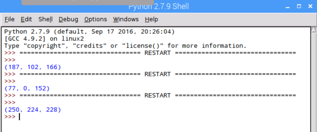
Xmin = 42, Xmax = 132, Xrange = 90

Ymin = 102, Ymax = 232, Yrange = 120

Zmin = 197, Zmax = 76, Zrange = 135

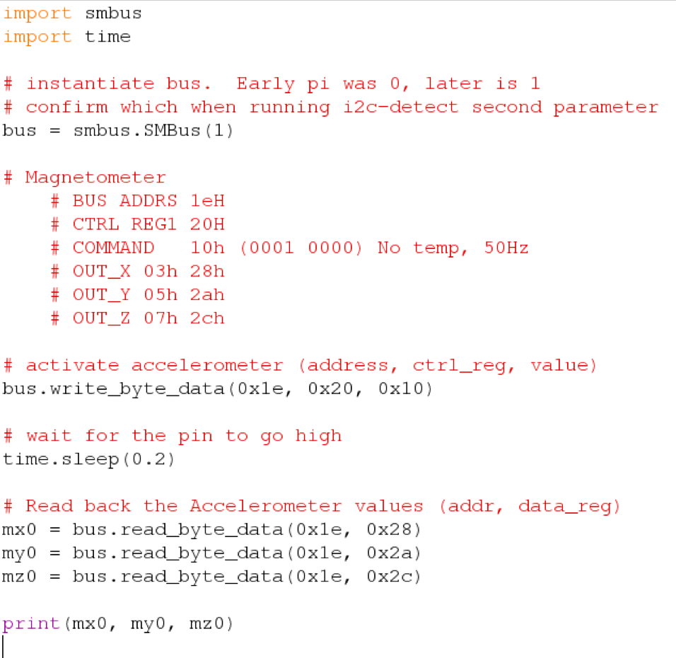
Now if one in the upper register is 360/256 degrees then that's maybe not too bad. Looks like I have some work to do with the MiniMu9 documentation to understand the readings.

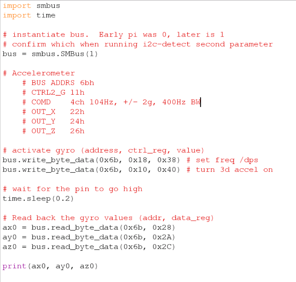
Here are the application notes for the compass chip.

"Understanding magnetic data The magnetic data are sent to the OUT_X_H, OUT_X_L, OUT_Y_H, OUT_Y_L, OUT_Z_H, and OUT_Z_L registers. These registers contain, respectively, the most significant part and the least significant part of the magnetic signals acting on the X, Y, and Z axes."

Not so helpful guys ... what do the numbers mean.

Let's resort to trial and error. With the device on the same table, rotating it 180 degrees to face South, here is the corresponding data:

It appears that my Y1 and Z1 values have not changed, but by rotating the device 180 degrees, my median X value has changed from 246/87 to 2/250. Now, assuming the lower register represents the 8 least significant bits of a 16 bit number

An alternative way of looking at this is that by rotating 180 degrees, the median magnetometer X reading has changed from (246*256)+87= 63,319 to (2*256) + 250 = 762.

OK, so I need to apply some scientific method. I've four questions that I wish to answer:

Is the compass behaving in a stable manner, or is it just sending random signals?
Does the compass signal behave in a way that is stable over the average of a series of readings, and if so, how long does the series have to be?
Is angular change represented linearly by the magnetometer readings?
How are the X, Y and Z axes oriented compared to horizontal and North?

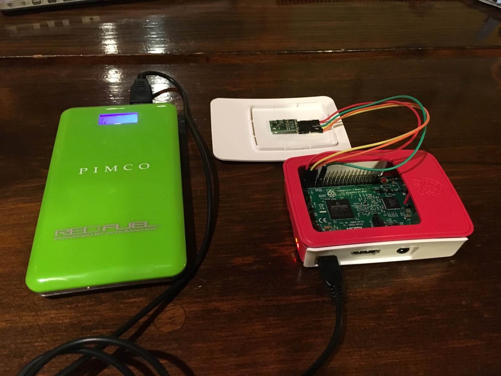
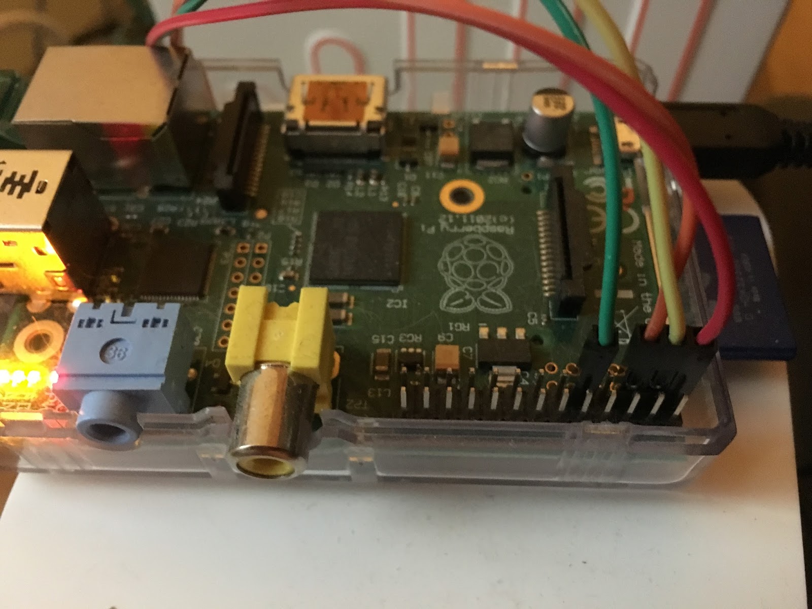
To research the answers to these questions I ran my Python code to collect a series of 200 readings with the Raspberry Pi oriented in 36 positions at 10 degree increments starting at North. The readings were taken on the same position on a smooth leveled surface. I measured the 10 degree increments using a military compass, as I noticed that the iPhone compass could jump by as much as 30 degrees without the iPhone being moved.

Ideally the data gathering would have been done on a carefully leveled surface, using a carefully calibrated turntable to rotate the sensor. I'm not expecting fantastic results, but let's take a look before I start spending on a calibration rig.

As the data were written to the SQLite database, the 10 degree run was assigned RUN_ID=17 with the RUN_IS incrementing by 1 until the 360 degree (North) run was assigned RUN_ID=52.

Analysis of Calibration Data

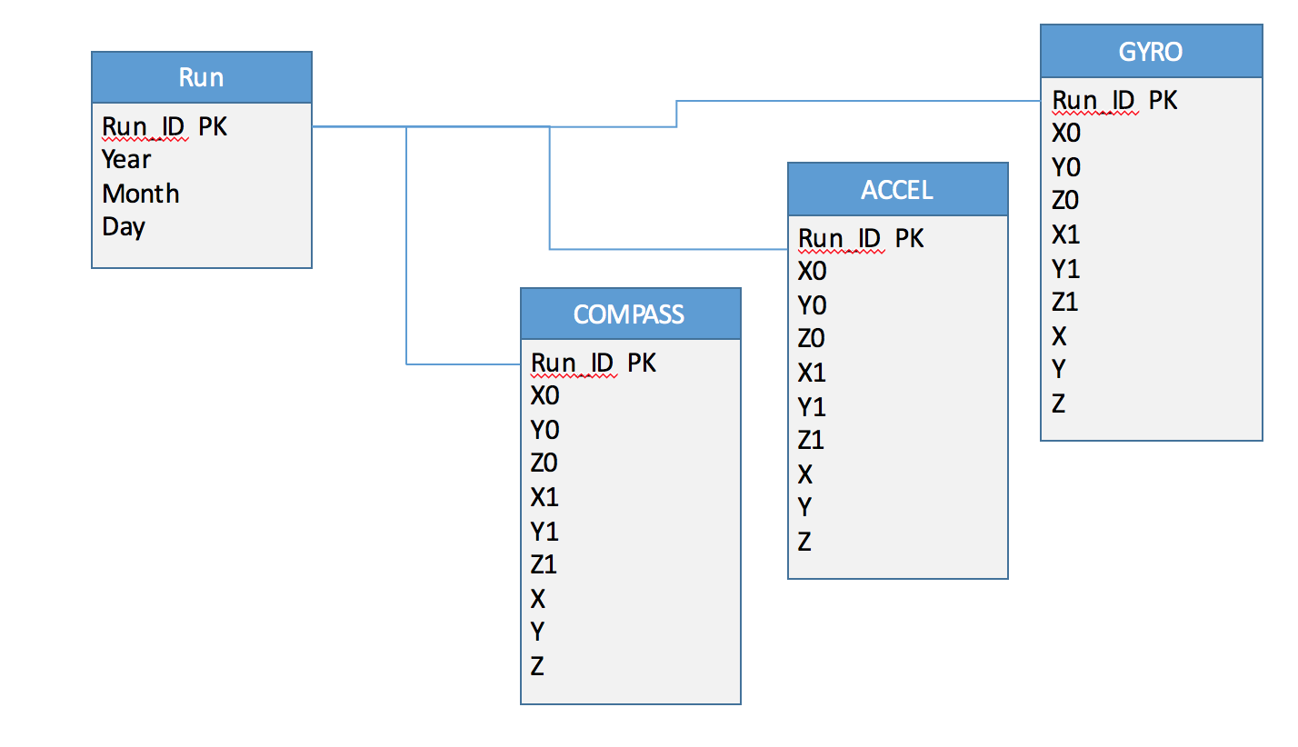
I took the data from the above runs and imported it into an R data frame using the RSQLite library:

library("RSQLite", lib.loc="~/Library/R/3.2/library")
library("ggplot2", lib.loc="~/Library/R/3.2/library")

c <- dbConnect(SQLite(),
dbname="/scratch/sqlite3/sensors.sqlite")

d <- dbGetQuery(c, "select * from compass where run_id >= 17")

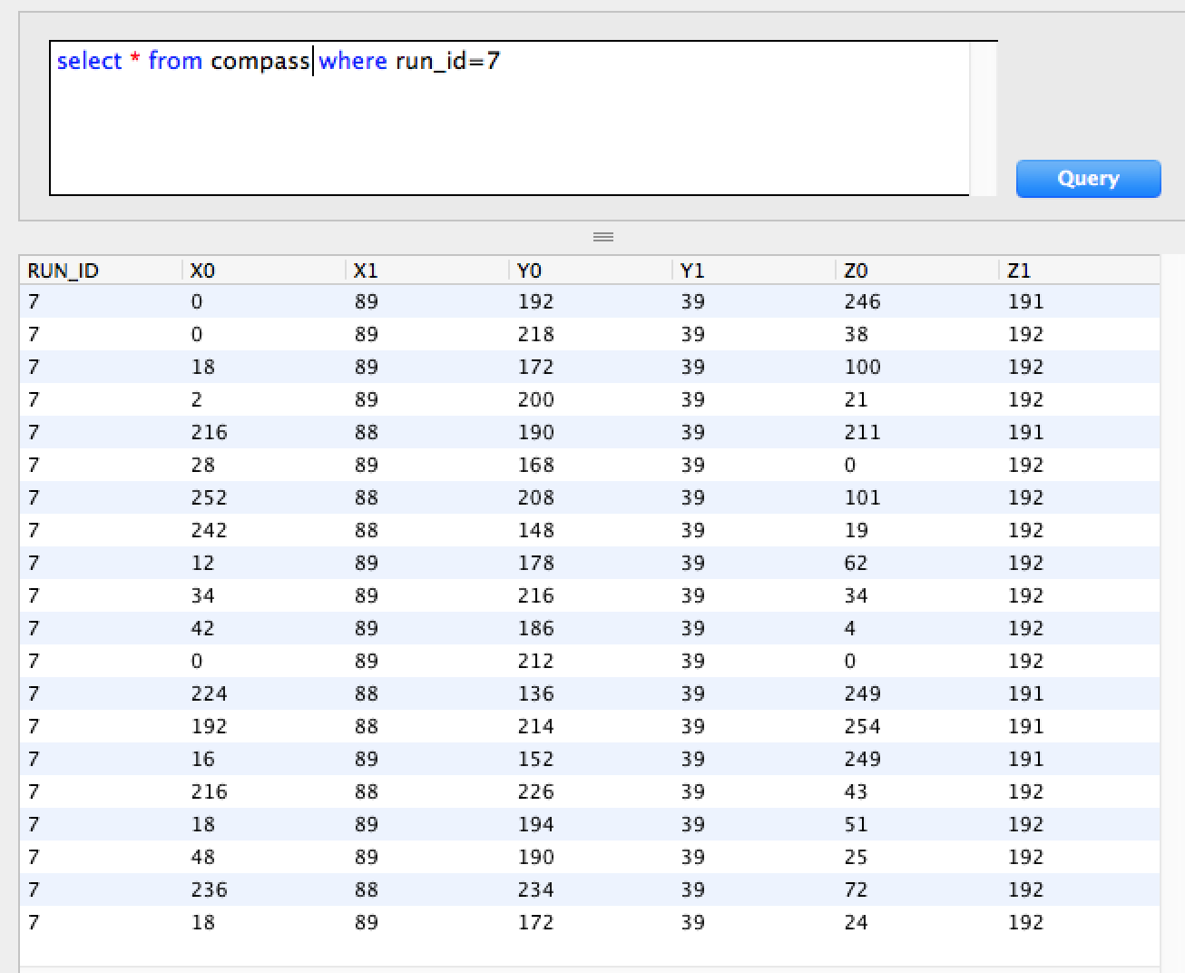
I then merged the values from the two registers, and adjusted the values where they had wrapped around 2^16 and started again at zero:

d$X <- (d$X1 * 256) + d$X0
d$Y <- (d$Y1 * 256) + d$Y0
d$Z <- (d$Z1 * 256) + d$Z0

# improve visibility by fixing the wrap around 2^16
d$X <- ifelse(d$X < 2^12, d$X + 2^16, d$X)
d$Y <- ifelse(d$Y < 2^12, d$Y + 2^16, d$Y)
d$Z <- ifelse(d$Z < 2^12, d$Z + 2^16, d$Z)

# Convert Run ID to a factor to improve color coding
d$RUN_ID <- factor(d$RUN_ID)

I then created a summary data set, showing the mean, median, sd, max and min values for each run.

library("plyr", lib.loc="~/Library/R/3.2/library")
Xsum <- ddply(d, "RUN_ID", summarize, Xavg=mean(X), Xmed=median(X), Xsd=sd(X), Xmin=min(X), Xmax=max(X), Xspread=max(X)-min(X))
Ysum <- ddply(d, "RUN_ID", summarize, Yavg=mean(Y), Ymed=median(Y), Ysd=sd(Y), Ymin=min(Y), Ymax=max(Y), Yspread=max(Y)-min(Y))
Zsum <- ddply(d, "RUN_ID", summarize, Zavg=mean(Z), Zmed=median(Z), Zsd=sd(Z), Zmin=min(Z), Zmax=max(Z), Zspread=max(Z)-min(Z))

# join dataframes
XYsum <- join(Xsum, Ysum, by="RUN_ID")
XYZsum <- join(XYsum, Zsum, by="RUN_ID")

Visualizations of Calibration Data

I then used ggplot2's qplot function to visualize the averages of X and Y for each set of readings. Ideally the data should form an ellipse. The shape of this ellipse will help us calibrate the compass.

qplot(data=XYZsum, x=Xmed, y=Ymed)

Note, the annotations were added using Affinity Designer and were not generated by qplot.

It's moderately elliptical. It's clear that the act of rotating skews the readings as there's a clear disconnect between the first and last readings. There are also potential sources of error arising from:

the compass reading
aligning the box of the Raspberry Pi with the edge of the compass
local magnetic variations (movement of people and objects close to the Raspberry Pi)
very large outlier readings which are skewing the mean.

To minimize the last of those problems I re-ran the chart using the median instead of the mean for each position of the Raspberry Pi. There really was not much difference between the two.

From here we should be able to draw a best fit ellipse through the data points, which can then be used to interpret future readings.

We can also repeat this for the XZ readings to interpret the angle in the XZ plane. The chipset documentation says that the Z axis is perpendicular to the plane of the board, which would make Z independent of rotation about the XY plane, which would result in a horizontal flat line. But we already know that the chip is mounted slightly off because the XY rotation resulted in an ellipse and not a circle. The XZ plot should therefore also result in an ellipse:

Again, not too pretty an ellipse, but for now lets assume that the errors arose from my non-scientific data gathering.

Before I do that, let's think about the variation in the readings within any given run, and how many readings we need to take to be sure we have an accurate compass reading.

Sampling Analysis

The first thing I noticed is that the Standard Deviations are quite small compared to the range. A typical example is the X readings for the 10 degree run. Of the two hundred readings:

the mean is 64,006.7
the median is 64,007
the standard deviation is 28.1
the minimum is 73 less than the median
the maximum is 75 more than the median

The readings are not widely dispersed, with all readings being within 3 standard deviations of the mean. Now, each of these readings was taken 0.1 seconds apart with the device standing still. My concern is that we will not have the opportunity to take a large number of readings spaced apart like this - a skier's direction will be rapidly changing. If I take a smaller number of readings more closely spaced, will I get a similar spread to calculate a good median without the skier moving too far during the sample? To test this I wrote a variation of the sampling code to take 30 samples immediately after each other.

Taking 30 samples only 0.1 seconds apart I get:

median is 65,778
the minimum is 34 less than the median
the maximum is 36 higher than the median

Reducing the sampling period to 0.01 seconds I get:

median is 65,809
the minimum is 57 less than the median
the maximum is 67 higher than the median

Eliminating the sample wait altogether I get:

median is 65,827
the minimum is 241 less than the median
the maximum is 207 higher than the median

I repeated this a number of times and the principle seems to hold, that if I do not wait between samples then I get bigger errors in the lower register. Increasing the wait to 0.5 seconds does not further reduce the error rate. Wait times in the range 0.05 - 0.1 seconds appear to have generally similar results.

It seems that I will have to accept inaccuracies in the direction measurement. If I take the median of ten samples 0.05 seconds apart, then I can only capture data every 0.5 seconds which is not sufficiently frequent for my needs. If I sample more frequently then the errors get larger, with the consequent risk that a small number of samples will not provide an accurate median. For now I will proceed with the approach of taking only a single sample of each reading, and having readings no closer than 0.05 Seconds apart, and will pay attention later to whether the noise in the readings detracts from the end result.

Fitting an Ellipse

Using the least squares fit method for fitting an ellipse to data, and the accompanying R code in Reference B, I fitted an ellipse to the data generated by the X and Y magnetometer sensors.

I found two problems with the results of the R code:

The angle of rotation is off by 90 degrees (pi/2 radians).
The fit is not particularly good when using large coordinates.

My sensor had created most values just below the maximum value of 2^16, but in a few cases had wrapped over the maximum 2^16 values and used values just over zero. I previously adjusted for this by adding 2^16 to any values that are less than 2^12. Because the ellipse matching works better with values centered on zero I now altered my coordinates by subtracting 2^16 from all of them.

I also arbitrarily added pi/2 to the angle of rotation to correct for that issue.

Incidentally, I encountered the same rotation issue when trying the Python code in Reference C. I also found with the Python code that the ellipsis semi-axes lengths were miscalculated with large coordinate values, and this issue was resolved when I subtracted 2^16 from all x and y values.

Here's my R code (I have not repeated the functions fit.ellipse and get.ellipse, which were used unaltered from the reference:

xy <- data.frame(XYZsum$Ymed, XYZsum$Xmed)

colnames(xy) <- c("x", "y")

xy$x <- xy$x - 2**16

xy$y <- xy$y - 2**16

xyfit <- fit.ellipse(x=xy$x, y=xy$y)

xyfit$angle += pi/2.0

xyElipseCoords <- data.frame(get.ellipse(fit = xyfit, n=360))

qplot(data = xy, x=xy$x, y=xy$y, color=I("red"), c(-2000, 1000), ylim = c(-7000, 4000) xlab = "x", ylab = "y") +

geom_point(data = xyElipseCoords, x=xyElipseCoords$x, y=xyElipseCoords$y, color="blue", shape=1)

And here's a plot of the original data in red and 360 data points on the fitted ellipse in blue:

Next I will take the 360 data points of the fitted ellipse and store them in a Python list with the point relating to North in the 360th position in the list. Thereafter, if I create a function to identify the closest point in the list to a sensor reading, then its position in the array will represent an angle in degrees in the XY plane, ie a compass heading.

I can also repeat this approach for the XZ plane and the YZ plane.

.import pandas as pd

def find_closest_pair(x, y, ref):
# ref is dict of the form {1: {x: 1, y: 2}, 2: {x: 3, y: 4}}
residuals = {}
for key in ref:
pt = ref[key]
residuals[key] = (pt["x"] - x)**2 + (pt["y"] - y)**2
min_error = min(residuals.values())
for key in residuals:
if residuals[key] == min_error:
min_error_posn = key
return [min_error_posn, min_error]

df = pd.read_csv("/Users/neildewar/scratch/xy360.csv")
ref = {}

for index, row in df.iterrows():
ref_pt = {}
ref_pt["x"] = float(row['x'])
ref_pt["y"] = float(row['y'])
ref[index] = ref_pt

closest = find_closest_pair(-1784, -1634, ref)

print(closest)

Now, that might be a lot of work to find out that True North is already stored in the last item in the array, but the function called find_closest_pair() will be re-used later on the Raspberry Pi when I need to match new sensor readings to return a direction in the XY plane.

References

A. Useful article on interpreting magnetometer readings: http://mythopoeic.org/magnetometer/

B. Article on best fitting an ellipse to data, providing R code: https://www.r-bloggers.com/fitting-an-ellipse-to-point-data/

C. Article on best fitting an ellipse to data, providing Python code: http://nicky.vanforeest.com/misc/fitEllipse/fitEllipse.html

Tuesday, December 27, 2016

Getting my Raspberry Pi mobile

In order to start using my sensors on the move I need to solve two mobility problems:

Provide a mobile power source (it's currently powered from mains)
Securing the sensor in the Raspberry Pi's case so that it's always in the same orientation to the case.

Mobile Power

I hunted around my office and found one of those cell phone emergency re-chargers that I had been given at a conference. The unit was a good sized one and should be able to run the Pi for a few hours. It's a RedFuel SL5.

The power unit comes with a cable that has a regular USB connector on one end, and a D port on the other end. It charges by plugging the USB end of the cable into a transformer, and the D connector into the port on the right of the above picture. When it's fully charged, the cable is turned around so that the USB end is plugged into the RedFuel power unit and the D connector is plugged into the Raspberry Pi's power port.

Securing the Sensor

To get consistent readings it will be important that the MiniMu-9 card is secured to the Raspberry Pi with a consistent orientation in all three dimensions. The MiniMu-9 board is not easily secured to the Raspberry Pi. I considered using an stand-off connector, but all four holes on the Raspberry Pi are used to secure it to its case. I decided to glue the cable connectors (not the board!) to the inside of the removable roof of the Rapsberry Pi. The cable coil away nicely inside the case. Here's the whole installation:

A SQL Database To Store The Data

Creating The Database

I used a copy of the Mac app SQLite Manager to create my database. I chose a simple relational model with four tables. The first table is to store details of the "run" ie a sequence of sensor readings. There are then three tables to store the actual readings from the gyro, accelerometer and compass respectively. Each of the three sensor tables includes a column that indicates the run that the sensor reading was associated with.

Each of the sensor tables contains six integer fields (X0, X1, Y0, Y1, Z0, Z1) to store the values that were read from the sensors. They also have three float fields (X, Y, Z) to store the numeric values after the readings have been processed and calibrated (more to follow on that later).

Writing Data to The Database

First a word of caution, close the SQLite Manager app before programmatically writing to a database. It has a nasty habit of crashing.

I wrote the Python code in Python 2.7.4 using the PyCharm Community Edition (ie free) IDE.

I have included python code below to write to the database. It is pretty straightforward. It uses three libraries:

The json library to parse the data that is stored in the data file.
The sqlite3 library to make the database connection to the sqlite database.
The os library allows interaction with the file system to change directory.

The python code then performs the following tasks:

Create the database connection
Open the JSON file that was created on the Raspberry Pi containing the sensor data
Read the JSON file and write it to the database tables

Read the header information to create a run record, and capture the RUN ID
Loop through the readings data, processing each in turn

Read Gyro data and write to DB
Read Accel data and write to DB
Read Compass data and write to DB

A few words on the sqlite code:

You initiate a connection to the database, that returns a connection object
The connection has a cursor object.
The cursor object is used to execute SQL commands against the database
The connection object is used to commit the SQL commands.

This website is very helpful on how to use the sqlite from Python.

import json
import os
import sqlite3


def init_db(db_file):
    conn = sqlite3.connect(db_file)
    return conn


def load_file(filename, filedir):
    os.chdir(filedir)
    f = open(filename, "r")
    d = json.load(f)
    return d


def process_header(header, db):
    c = db.cursor()
    # expects dict of the form {"type": "header", 
                             #  "Month": 12, 
                             #  "Day": 4, 
                             #  "Year": 2016}
    c.execute("INSERT INTO RUN (Year, Month, Day) 
              "values ({yr}, {mth}, {day})".
        format(yr=header["Year"], 
               mth=header["Month"], 
               day=header["Day"]))
    db.commit()
    return c.lastrowid  # return the PK of the last row entered

def process_reading(reading, db, header):
    c = db.cursor()
    accel = reading["accel"]
    c.execute("INSERT INTO ACCEL (RUN_ID, x0, x1, y0, y1, z0, z1) "
              "values ({hdr}, {x0}, {x1}, {y0}, {y1}, {z0}, {z1})".
        format(hdr=header,
               x0=accel["x0"],
               x1=accel["x1"],
               y0=accel["y0"],
               y1=accel["y1"],
               z0=accel["z0"],
               z1=accel["z1"]))
    db.commit()

    gyro = reading["gyro"]
    c.execute("INSERT INTO GYRO (RUN_ID, x0, x1, y0, y1, z0, z1) "
              "values ({hdr}, {x0}, {x1}, {y0}, {y1}, {z0}, {z1})".
        format(hdr=header,
               x0=gyro["x0"],
               x1=gyro["x1"],
               y0=gyro["y0"],
               y1=gyro["y1"],
               z0=gyro["z0"],
               z1=gyro["z1"]))

    db.commit()

    compass = reading["magno"]
    c.execute("INSERT INTO COMPASS (RUN_ID, x0, x1, y0, y1, z0, z1)"
              " values ({hdr}, {x0}, {x1}, {y0}, {y1}, {z0}, {z1})".
        format(hdr=header,
               x0=compass["x0"],
               x1=compass["x1"],
               y0=compass["y0"],
               y1=compass["y1"],
               z0=compass["z0"],
               z1=compass["z1"]))
    db.commit()


def json_to_sql(readings, db):
    header_id = process_header(readings["header"], db)
    for element in readings:
        item = readings[element]
        if item["type"] == "reading":
            process_reading(item, db, header_id)

db_conn = init_db("/sqlite3/sensors.sqlite")
sensor_data = load_file("readings.data",

             "/scratch/Raspberry.Pi/sensor_data")
json_to_sql(sensor_data[0], db_conn)

The results stored in the SQLITE database are shown below

More to follow later on this as I explore the meaning of the captured data.

Saturday, November 26, 2016

Python Code To Record Sequence

Many uses of chip sets like the MiniMu9 are for robotics, so it's necessary to convert the readings into valuable properties like pitch and yaw. Whilst that may be useful down the road, because I don't plan to handle the data in real time I want to simply capture the data and store it for offline processing. I therefore must write Python code that will read each sensor in turn, and write the data to a file on the Raspberry Pi's USB drive.

Requirements

Here are my requirements for the code:

Take a parameter for the number of seconds to run the sampling (this will subsequently be replaced with start/stop switch)
Sample each of the three devices in sequence
Write the data to arrays
At the end of the run, write the arrays to a json file for offline reading

Format of the json file:

[
   {
    "header" = {"type": "header", "Month": 12, "Day": 4, "Year": 2016},
    "r1" = {"type": "reading",
            "timestamp": {"Second": 39, "Microsecond": 998934, "Minute": 34, "Hour": 12},
            "gyro": {"y0": 162, "x0": 7, "z0": 162}, "id": 0,
            "accel": {"y0": 171, "x0": 21, "z0": 161},
            "magno": {"y1": 255, "y0": 56, "x0": 46, "x1": 5, "z0": 110, "z1": 4}
           },

...
    "r2" = {"type": "reading",
            "timestamp": {"Second": 40, "Microsecond": 39239, "Minute": 34, "Hour": 12},
            "gyro": {"y0": 161, "x0": 255, "z0": 162}, "id": 1,
            "accel": {"y0": 170, "x0": 1, "z0": 158},
            "magno": {"y1": 255, "y0": 72, "x0": 20, "x1": 5, "z0": 66, "z1": 4}
           }

Rationale

I want to write this code and review the resulting data with three objectives in mind:

Calibrate each of the sensors - work out what needs to be added or subtracted to get to zero,
Work out how stable the data is from each of the 9 sensors - I will do statistical analysis of the data sets arising from the sensors.
Based on (2.) work out how to combine data from the accelerometer and gyro to get an accurate reading (by combining them and also by taking a trailing average to smooth erratic readings)

Python Code

import smbus
import datetime
import os
import time
import json


def get_magnetometer():
    # activate Magnetometer (address, ctrl_reg, value)

    bus.write_byte_data(0x1e, 0x20, 0x10) 
    bus.write_byte_data(0x1e, 0x21, 0x00)
    bus.write_byte_data(0x1e, 0x22, 0x00) 
    time.sleep(0.01)
    readings_m = dict()
    # Read back the Magnetometer values (addr, data_reg)

    readings_m["x0"] = bus.read_byte_data(0x1e, 0x28)
    readings_m["x1"] = bus.read_byte_data(0x1e, 0x29)
    readings_m["y0"] = bus.read_byte_data(0x1e, 0x2a)
    readings_m["y1"] = bus.read_byte_data(0x1e, 0x2b)
    readings_m["z0"] = bus.read_byte_data(0x1e, 0x2c)
    readings_m["z1"] = bus.read_byte_data(0x1e, 0x2d)

    return(readings_m)


def get_gyro():
    # activate gyro (address, ctrl_reg, value)

    bus.write_byte_data(0x6b, 0x16, 0x38)
    bus.write_byte_data(0x6b, 0x11, 0x40)
    time.sleep(0.01)
    readings_g = dict()
    # Read back the gyro values (addr, data_reg)

    readings_g["x0"] = bus.read_byte_data(0x6b, 0x22)
    readings_g["x1"] = bus.read_byte_data(0x6b, 0x23)
    readings_g["y0"] = bus.read_byte_data(0x6b, 0x24)
    readings_g["y1"] = bus.read_byte_data(0x6b, 0x25)
    readings_g["z0"] = bus.read_byte_data(0x6b, 0x26)

readings_g["z1"] = bus.read_byte_data(0x6b, 0x27)
    
    return(readings_g)


def get_accel():
    # activate accel (address, ctrl_reg, value)

    bus.write_byte_data(0x6b, 0x18, 0x38) # set freq /dps

    bus.write_byte_data(0x6b, 0x10, 0x40) # turn 3d accel on

    time.sleep(0.01)
    readings_a = dict()
    # Read back the gyro values (addr, data_reg)

    readings_a["x0"] = bus.read_byte_data(0x6b, 0x28)
    readings_a["x1"] = bus.read_byte_data(0x6b, 0x29)
    readings_a["y0"] = bus.read_byte_data(0x6b, 0x2A)
    readings_a["y1"] = bus.read_byte_data(0x6b, 0x2B)
    readings_a["z0"] = bus.read_byte_data(0x6b, 0x2C)
    readings_a["z1"] = bus.read_byte_data(0x6b, 0x2D)





return(readings_a)


def write_data(filename, data):
    # assumes directory already set in main (avoids repeated sets)    f = open(filename, "w")
    json.dump(data, f)
    f.close()
   
## Maintry: os.chdir("/usbdrv/data/sensor_data")
except: os.mkdir("/usbdrv/data/sensor_data")
# confirm which when running i2c-detect second parameterbus = smbus.SMBus(1)

dt = datetime.datetime

# wait for the pin to go high
header = dict()
header["type"] = "header"header["Year"] = dt.today().year
header["Month"] = dt.today().month
header["Day"] = dt.today().day

file_data = dict()
file_data["header"] = header

for i in (range(0, 20)):
    timestamp = dict()
    timestamp["Hour"] = dt.today().hour
    timestamp["Minute"] = dt.today().minute
    timestamp["Second"] = dt.today().second
    timestamp["Microsecond"] = dt.today().microsecond

    readings = dict()
    readings["type"] = "reading"    readings["id"] = i
    readings["timestamp"] = timestamp
    readings["magno"] = get_magnetometer()
    readings["gyro"] = get_gyro()
    readings["accel"] = get_accel()
    file_data["r" + str(i)] = readings

to_json = [file_data]  # encapsulate dict in list
print(file_data)

write_data("readings.data", to_json)

Wednesday, September 21, 2016

Programming the i2c Bus in Python

Reference

There's a useful reference on the Raspberry Pi website targeted at kids using the Raspberry Pi, that has a tutorial on GPIO programming in Python.

Python

To program the Raspberry Pi I chose to use Python 2.7.4 which was pre-installed with the JESSIAN Linux OS. I wrote and tested the code using the simple Idle IDE application which came pre-installed with the Raspberry Pi's Linux operating system. Be sure to use the correct version of Idle ... Idle is for Python 2.7 and Idle3 is for Python 3.0.

When I wrote the final code I also worked in the PyCharm IDE on my Mac because I like its code formatting features. PyCharm can be used to edit code on a different computer using SSH.

Python's smbus Library

The first thing I had to do before beginning to code was to install the Python smbus library, which provides a high level abstraction from the specific pin voltages that need to be set to communicate on the i2c bus. It's important to note here that I'm using Python 2.7 and the Idle IDE (ie not Idle 3 which is for Python 3.x). The smbus library does not install the same way with Python 3, and may need manual packaging).

This was installed from the Raspberry Pi's Linux command line using:

sudo apt-get install python-smbus

The smbus library when used in python has three important commands:

bus = smbus.SMBus(n)
... is used to instantiate an smbus object that can then be used to execute commands. From reading various articles, early Raspberry Pi devices used n=0, and later ones used n=1. This is the same value that is passed in the i2c-detect command, which by trial and error I worked out should be n=1.

Once the smbus object has been instantiated, there are commands to write and read data to / from the bus.

To activate a device on the bus, we must write to its control register. The command to do this is:
bus.write_byte_data(bus_address, control_register, value)

To read data from a device we use:
bus.read_byte_data(bus_address, data_register)

Checking For Responses

Next I wrote three short scripts to sample each of the sensors and print out the results.

Accelerometer:

Gyroscope:

Magnetometer / Compass

Results:

Fantastic! I'm now reading values from all three devices, so now I can write a some useful code to capture a sequence of readings.

Reference

The most helpful reference for this project has been Ozzmaker. It certainly does not provide a straight lift-out for two reasons - this blog uses a different sensor board, and programs in C rather than my preferred Python.

Exploring the i2c Bus

In this project I am using three separate sensor chips that are built into the AltiMU-10 sensor board: Gyro, Accelerometer and Magnetometer. By careful review of the the documentation on the Pololu web page for the MiniMu-9 V5

MiniMu9

The MiniMu9 circuit board contains three devices, a gyro, a magnetometer and a compass. Each of the three devices has three sub sensors, X, Y and Z each representing a different dimension / orientation.

We communicate with the MiniMu9 using the Raspberry Pi's i2c serial bus. The i2c bus is a serial bus that allows a computer to communicate with a variety of devices connected to the bus. Broadly, this is how it works:

Each device has an address on the bus
Each device has a set of registers which can either be readable, writable or both
Some of the registers are control registers, where you can read or write settings
Some of the registers are data registers, where you can read or write data

A reading from one of the 9 sensors is read by sending a value to a register to tell the circuit which value we wish to read, then reading the value from a specific address. We will need to read all nine addresses in order to take one complete set of readings.

Physical Connectivity

The i2c bus is accessed through the Raspberry Pi's serial input/output port. 4 wire connections are needed as follows:

Raspberry Pi Port Altimu-10 Port Purpose My Cable Color

1 3V VDD 3V Power Red

3 GPIO-0 SDA SDA Yellow

5 GPIO-1 SCL SCL Orange

9 Ground GND GND Black

The picture above shows the orientation of the pin-out on the Raspberry Pi (note, this is picture of the Raspberry Pi V2 - I will retake the pic with a V3).

Raspberry Pi i2c Bus

i2c bus is a software convention for multiple devices to communicate with a computer over the same serial bus. The Raspberry Pi's General Purpose Input Output (GPIO) connector (bottom right in the picture above) communicates with the Pi's processor using i2c.

The i2c bus documentation is available online, though is generally not needed here as the developer is abstracted from the complexities the electronic circuits by using a software library. More to follow on the software later.

First, check that the i2c capability is enabled by accessing the Raspberry Pi's configuration menu:
sudo raspi-config

From the menu select Advanced Options, then select I2C. On the next screen you are asked if you wish to enable the ARM I2C interface - select YES.

Reboot the Raspberry Pi to make the I2C interface active.

Next install the package that allows Python to communicates with the bus:

sudo apt-get install python-smbus

Next I install i2c tools, a package that allows you to see if devices are active on the i2c bus using the i2cdetect application. From the Linux command line:
sudo apt-get install i2c-tools libi2c-dev

After saving and exiting from Nano, the Raspberry Pi must be rebooted from the command line with:
sudo reboot

Testing The i2c Bus

After rebooting I can use i2c tools to identify if the connections are working correctly. From the Linux command line I run:
sudo i2cdetect -y 1
The resulting grid is displayed:

I see the device addresses 6bH and 1eH are visible on the ic2 bus, and that no others are visible. I check that against the port addresses used by the Gyro, Accelerometer and Magnetometer from my device documentation. This looks good as the Gyro and Accelerometer both use 6b and the compass uses 1e.

Port Addresses

Gyro - LSM6DS33

Address 0x6b
Control Register 2_G 0x11
Message 0x40 01000000b 104Hz, 245dps, Gyro full scale at 125dps
Control Register 7_G 0x16
Message 0x38 00111000b - X, Y, Z Gyro on
X Data Low 0x22
X Data High 0x23
Y Data Low 0x24
Y Data High 0x25
Z Data Low 0x26
Z Data High 0x27

Accelerometer - LSM6DS33

Address 0x6b 1101011b
Control Register 1XL 0x10
Message 0x40 01000000b - 104Hz, +/- 2g, 400Hz BW
Control Register 9XL 0x18
Message 0x38 00111000b - X, Y, Z Accel on
X Data Low 0x28
X Data High 0x29
Y Data Low 0x2a
Y Data High 0x2b
Z Data Low 0x2c
Z Data High 0x2d

Magnetometer - LIS3MDL

Address 0x1e
Control Register 1 0x20
Message 0x10
Control Register 4 0x23
Message 0x00
X Data Low 0x28
X Data High 0x29
Y Data Low 0x2a
Y Data High 0x2b
Z Data Low 0x2c
Z Data High 0x2d
Temp Low 0x2e
Temp High 0x2f

Raspberry Pi Basics

I started out with a new (Dec 2016) Raspberry Pi v3 purchased online from Amazon. When I first tried this project I spent a lot of time getting basic functions like WiFi working. The new Pi has onboard wifi and bluetooth, which makes things much easier, as the Linux OS is preconfigured to use them.

The Raspberry Pi comes without an operating system, and without any storage. It has a Micro-SD slot and four USB ports. It is configured to boot from an operating system on the Micro-SD slot. Best practice is to put the operating system on a fast Micro-SD card, and use a USB thumb drive to store data.

Operating System Installation

Any Linux OS will work on the Raspberry Pi, but it is best to use a variant that has been built specifically for the Raspberry Pi. I chose the most common on which is called Raspbian. Raspbian has named major releases, the first was called Debian, the second and latest is called Jessian.

The operating system is downloaded from the Raspberry Pi website. There are two sets of installation files to choose from: "New Out of The Box" aka NOOBS, which is a simple version with everything pre-configured, and a version to self-configure. I chose NOOBS. Here are the steps:

Download NOOBS to my Macbook
Unzip the NOOBS download
Insert the SD card into my Macbook
Using the Mac Disk utility format the SD card as MSDOS
Using Finder, copy the NOOBS files into the root directory of the SD card
Put the SD card into the Raspberry Pi's SD card slot. Connect keyboard, mouse and monitor and boot it.
The Raspberry Pi presents a configuration screen. I selected Raspberry Pi "JESSIAN" operating system full version, and English-US keyboard. I did not configure WiFi at this stage. The software then proceeded to install and configure itself and booted up to a Linux desktop.

Configuring WiFi on a Rapsberry Pi 3 with JESSIAN is easy. No editing of files like the previous version, just click the WiFi icon, select the network SSID, enter the network password and you are done.

With the wifi now working, I want to set the PC up for remote access. I want two types of remote access: SSH terminal access and RealVNC screen sharing. I will do the SSH first, as once I have that I can configure the Raspberry Pi for RealVNC remotely over SSH.

The Raspberry Pi comes with a default user account called "pi" with a password of "raspberry". First thing to do is to reset the password for the account pi. This can be done by opening a terminal window on the Pi and using the passwd linux command. Note that you will be forced to select a complex password that is not based on a dictionary word.

Static IP Address

Because I don't want to have to reconfigure my SSH and VNC settings each time the Raspberry Pi device is assigned a new IP address by DHCP, the next thing to do is to configure the Raspberry Pi for a static IP address. This involves two steps: (1) reserve an IP address for the Raspberry Pi on the router and (2) configure the reserved IP address on the Raspberry Pi.

For my router I'm using an airport extreme, so I open the Airport Utility, select the Airport, select Edit. On the network tab I add a DHCP reservation for the Raspberry Pi. I chose 192.168.0.30

The Raspberry Pi's Static IP address on the WiFi interface is configured by editing the file /etc/dhcpcd.conf and adding the following lines at the end:

interface wlan0

static ip_address=192.168.0.200/24 static routers=192.168.0.1 static domain_name_servers=192.168.0.1

Secure Shell (SSH)

I enable the Raspberry Pi's SSH server. On the Raspberry Pi terminal window, run the rasbpi-config command. Select "Advanced Options" then enable both SSH.

If I open a terminal window on my Mac I can run:
ssh pi@192.168.0.23
I am then prompted for a password and I am able to enter script commands directly to the Raspberry Pi.

Configure USB Drive For Storage

Here's a good Instructable on setting up the USB drive. It was straightforward to follow. After formatting it I created two directories in the USB drive root - /code and /data. When I configured the USB drive into the Raspberry Pi file system I made it /usbdrv, so on the Pi the directories will appear as /usbdrv/code and /usbdrv/data. I also made a second mapping so that my code and data folders would appear under /home/pi/usb.

File Transfer

To be able to easily transfer files between my Macbook and the Raspberry Pi, I use the Macbook's Finder app and configure the Raspberry Pi as a remote server by selecting
Go / Connect to Server

The Raspberry Pi's file system is now visible in the Finder left nav in the "Shared" section. I am able to navigate to the /usbdrv folder which represents the USB drive that is plugged into the Raspberry Pi.

In the dialog that appears I add afp://192.168.0.23, and when prompted I enter the username pi and the password that I changed on the Raspberry Pi.

Remote Desktop (VNC)

To remotely control the Raspberry Pi's desktop requires three tasks

Enable the VNC server function on the Raspberry Pi's BIOS
Set the VNC server running
Run VNC client software on my Mac and make a connection to the Raspberry Pi

I enable the Raspberry Pi's VNC server. On the Raspberry Pi terminal window, run the rasbpi-config command. Select "Advanced Options" then enable both SSH.

To set the VNC server running, run the following command:

vncserver :1 -geometry 1024x600 -depth 16 -pixelformat rgb56

Next to access the remote desktop on the Raspberry Pi. I downloaded the Mac VNC viewer application from the RealVNC website. I launch the app and enter the details of the Raspberry Pi
192.168.0.23:5901

Note - the password entered is not the password associated with the Pi account on the Raspberry Pi - it is the password that was entered as the VNC password when VNC was installed on the Raspberry Pi.

I am now able to remotely control the Raspberry Pi's desktop (of course being careful to use the Mac's Control Key instead of the Command Key!)

Next Steps

Once all that's in place then I can move on to the new sensor board, and accessing it via the Raspberry Pi's i2c Serial Bus.